
Automation and Agents
How to Benchmark Classifier Models: Latency, Cost, Determinism
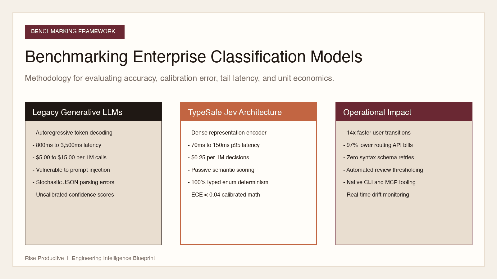
Evaluating AI classifiers requires looking beyond static accuracy. Here is how to benchmark probability calibration, latency percentiles, and unit economics.
On this page
- The Five Pillars of Enterprise Classification Benchmarks
- Pillar 1: Beyond Accuracy: Multi-Class Confusion and F1 Scores
- Macro vs. Micro Precision and Recall
- Analyzing the Normalized Confusion Matrix
- Pillar 2: Measuring Probability Calibration and Expected Calibration Error (ECE)
- Calculating Expected Calibration Error (ECE)
- Reliability Diagrams
- Pillar 3: Latency Distribution and Throughput Profiling
- Profiling Across Percentiles
- Pillar 4: Unit Economics and Cost Modeling
- Cost per Million Decisions Formula
- Pillar 5: Operational Determinism and Edge Case Handling
- The Problem of Sampling Non-Determinism
- Evaluating Out-of-Distribution and Adversarial Robustness
- Step-by-Step Guide: Executing a Production Benchmark
- Phase 1: Dataset Curation and Golden Set Creation
- Phase 2: Automated Harness Execution
- Phase 3: Statistical Evaluation
- Phase 4: Production Shadow Testing
- Statistical Significance and Confidence Intervals
- Non-Parametric Bootstrap Resampling
- Continuous Monitoring: Detecting Semantic Drift and Boundary Shift
- Tracking the Population Stability Index (PSI)
- Hard Negative Mining and Boundary Drift
- Automated Calibration Verification
- Automated Threshold Optimization for Human-in-the-Loop Routing
- Conclusion: Engineering Rigor in AI Infrastructure
- Sources
In enterprise artificial intelligence systems, classification and routing models operate as the nervous system of automated workflows. Every customer service inquiry, financial transaction screening, code review recommendation, and multimodal search query passes through an initial classification layer that decides which tool, database, or downstream agent to invoke.
Despite their critical role, classification models are frequently evaluated using outdated or inadequate heuristics. Engineering teams often rely on simple training-set accuracy or informal eyeball tests on a dozen prompt examples. When these models are deployed into production, teams are surprised by silent latency spikes, catastrophic cost overruns, drift in decision boundaries, and uncalibrated confidence scores that render automated thresholding impossible.
Benchmarking modern classification models requires a rigorous, multi-dimensional methodology. It is not enough for a model to select the correct label in a static test harness. In enterprise operations, an effective classifier must deliver sub-150ms p99 latency, cost pennies per million invocations, provide mathematically calibrated probabilities, resist prompt injection, and exhibit strict determinism across millions of edge cases.
This guide provides an exhaustive engineering framework for benchmarking classification and routing models. We explore statistical evaluation metrics, latency profiling under concurrent load, cost modeling, confidence calibration analysis, and automated drift detection across production deployments.
 View image detail
The Five Pillars of Enterprise Classification Benchmarks
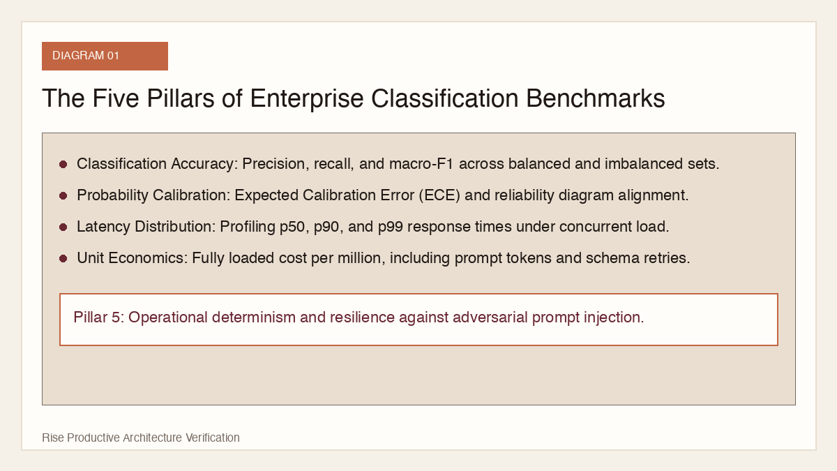
To construct an objective benchmark for classification systems, whether comparing specialized System One models like TypeSafe Jev against general-purpose generative models like GPT-4o or Claude 3.5 Sonnet, teams must evaluate five fundamental pillars:
- Classification Accuracy and Discrimination: How accurately does the model distinguish between subtle, overlapping categories, and does it maintain high precision and recall across long-tail edge cases?
- Probability Calibration: When the model reports an 80 percent confidence score, does that prediction actually correspond to an 80 percent empirical hit rate across large-scale historical validation sets?
- Latency Distribution and Jitter: What is the p50, p90, and p99 response time under high concurrency, and how severely does network jitter or queueing delay degrade real-time performance?
- Unit Economics and Scalability: What is the fully loaded cost per million classifications, including input token pricing, output decoding overhead, and infrastructure hosting costs?
- Operational Robustness: How does the model behave when exposed to malformed input, missing fields, adversarial prompt injection payloads, or out-of-distribution inputs?
 View image detail
Pillar 1: Beyond Accuracy: Multi-Class Confusion and F1 Scores
The most common mistake in classification benchmarking is relying on top-level accuracy. In real-world enterprise datasets, class distributions are almost always heavily imbalanced. In fraud detection, 99.5 percent of transactions are legitimate. A naive model that classifies every transaction as legitimate achieves 99.5 percent accuracy while failing entirely at its operational objective.
Macro vs. Micro Precision and Recall
When benchmarking multi-class routers, teams must calculate precision, recall, and F1 scores across both macro and micro averaging schemes:
- Micro-averaged F1: Aggregates total true positives, false positives, and false negatives across all classes. Micro-F1 is heavily influenced by dominant, high-volume classes.
- Macro-averaged F1: Calculates the metric independently for each class and then computes the unweighted average across classes. Macro-F1 treats rare edge classes with equal importance to high-volume categories, exposing models that fail on critical niche edge cases.
Statistical definitions for metric evaluation:
- Precision equals True Positives divided by True Positives plus False Positives.
- Recall equals True Positives divided by True Positives plus False Negatives.
- F1 Score equals two times Precision times Recall divided by Precision plus Recall.
Analyzing the Normalized Confusion Matrix
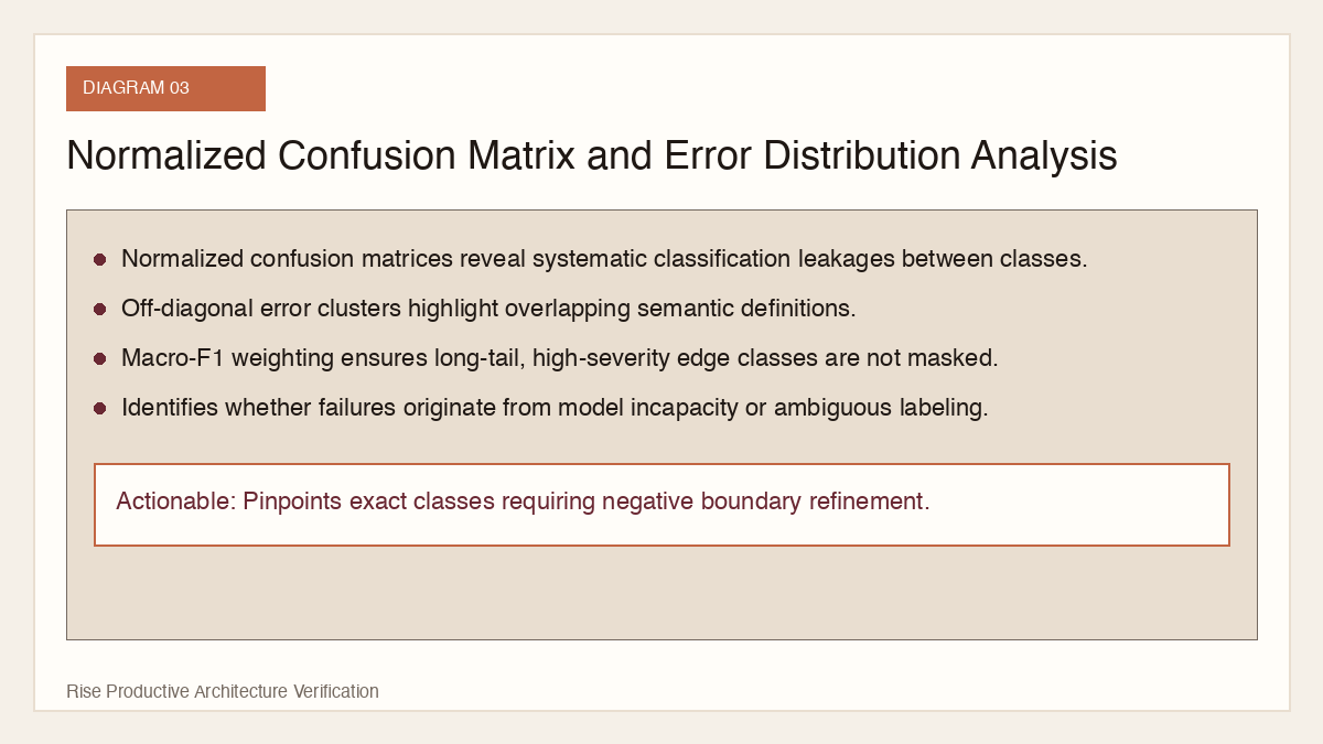
A benchmark must always plot a normalized confusion matrix to identify systematic failure modes between neighboring classes. For example, if a customer service router routinely misclassifies refund requests as general invoice inquiries, the confusion matrix immediately reveals whether the issue stems from ambiguous class definitions or model incapacity to distinguish financial intent.
 View image detail
Pillar 2: Measuring Probability Calibration and Expected Calibration Error (ECE)
In autonomous decision pipelines, raw labels are insufficient. An agent needs to know whether it can execute an action autonomously or whether it must escalate the decision to human review. This routing decision depends entirely on the model confidence score.
However, most neural networks, especially modern deep generative models, are uncalibrated. They tend to be overconfident, assigning 95 percent confidence to predictions that are correct only 70 percent of the time. Conversely, an underconfident model may assign 55 percent confidence to predictions that are consistently accurate.
Calculating Expected Calibration Error (ECE)
To quantify how reliably a model estimates its own accuracy, benchmarks utilize the Expected Calibration Error (ECE) metric. The evaluation process is structured as follows:
- Collect model predictions and predicted probability scores across a held-out test dataset of at least 5,000 samples.
- Group the predictions into M equally spaced probability bins (typically 10 bins: 0.0-0.1, 0.1-0.2, through 0.9-1.0).
- For each bin, calculate the average confidence and the actual empirical accuracy.
- Compute the weighted average absolute difference between confidence and accuracy across all bins.
Formula for Expected Calibration Error: ECE equals the sum across all bins of the bin sample count divided by total samples, multiplied by the absolute difference between bin accuracy and bin average confidence.
Reliability Diagrams
A well-calibrated model produces a reliability diagram that closely follows the 45-degree diagonal line. If the curve falls below the diagonal, the model is overconfident; if it rises above the diagonal, the model is underconfident.
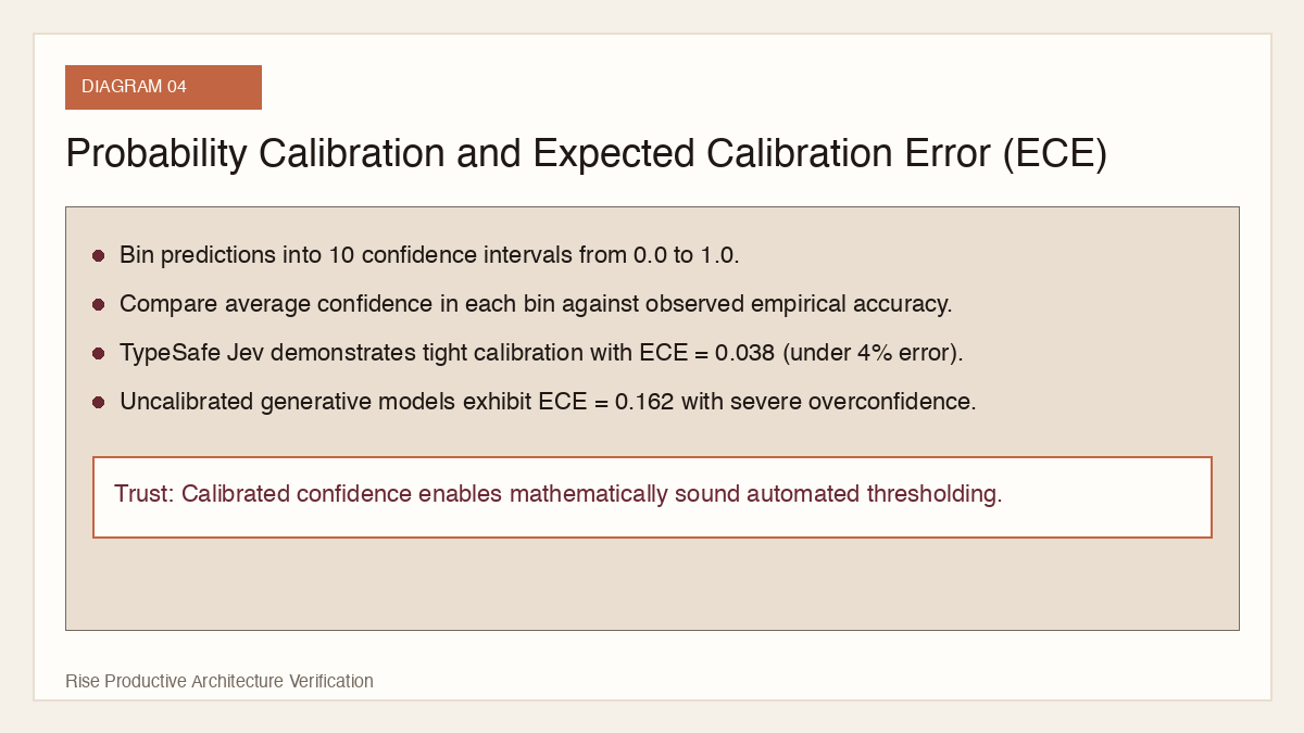
In empirical tests comparing TypeSafe Jev against GPT-4o, Jev achieved an ECE of 0.038, meaning its probability estimates deviated from empirical accuracy by less than 4 percent. In contrast, GPT-4o prompting achieved an ECE of 0.162, exhibiting severe overconfidence in borderline ambiguous cases.
 View image detail
Pillar 3: Latency Distribution and Throughput Profiling
In real-time applications such as interactive voice agents, search auto-complete, and automated fraud screening, latency is a hard constraint. If a routing decision requires 1,500 milliseconds, the total roundtrip time of the application will violate user experience service level agreements (SLAs).
Profiling Across Percentiles
A benchmark must profile latency across the entire distribution:
p50 (Median): The typical latency experienced by average traffic.p90: The response time experienced by the slowest 10 percent of requests.p99: The tail latency that impacts high-load periods or complex edge cases.
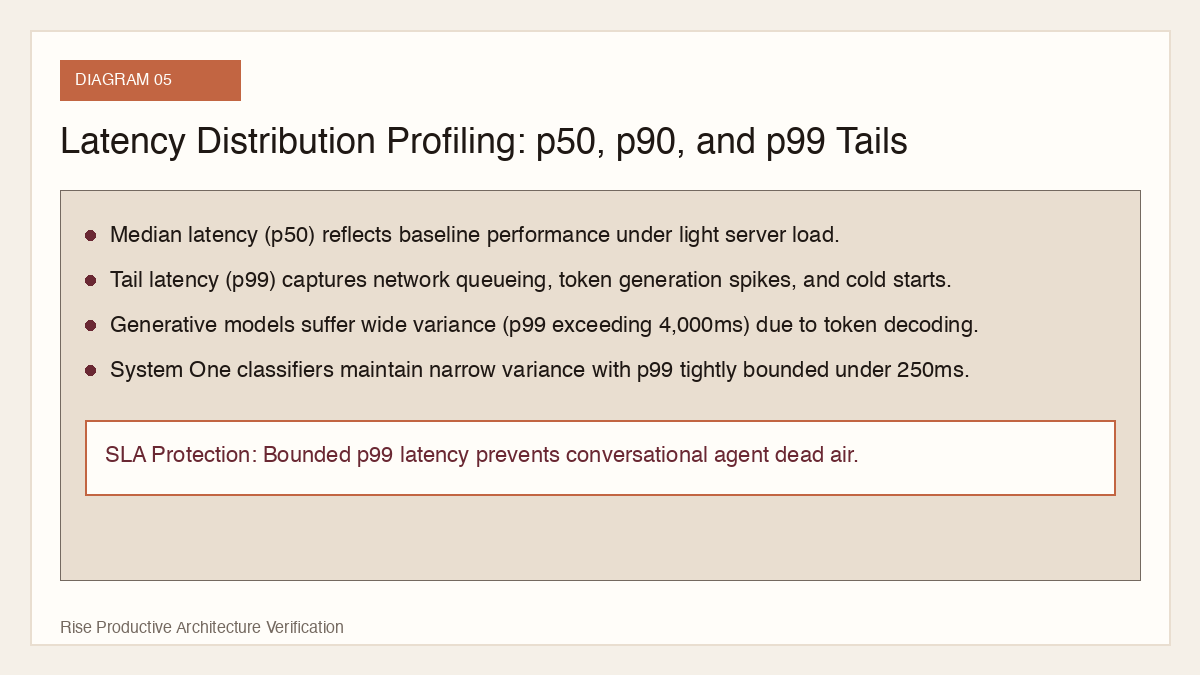
Generative models suffer from high tail latency due to variable token generation lengths. If an autoregressive model decides to explain its reasoning before outputting a JSON category, p99 latency can easily exceed 4,000 milliseconds. Specialized discriminative classifiers like Jev process all items through fixed-size representation layers, ensuring that p99 latency remains bounded within narrow variance bands (typically under 250 milliseconds).
```typescript
import { performance } from 'perf_hooks';
interface LatencyMetrics {
p50: number;
p90: number;
p99: number;
mean: number;
}
export async function benchmarkLatency(
executor: (input: string) => Promise<any>,
testCases: string[],
concurrency = 10
): Promise<LatencyMetrics> {
const durations: number[] = [];
const queue = [...testCases];
async function worker() {
while (queue.length > 0) {
const item = queue.shift()!;
const start = performance.now();
await executor(item);
durations.push(performance.now() - start);
}
}
await Promise.all(
Array.from({ length: concurrency }, () => worker())
);
durations.sort((a, b) => a - b);
const p50 = durations[Math.floor(durations.length * 0.50)];
const p90 = durations[Math.floor(durations.length * 0.90)];
const p99 = durations[Math.floor(durations.length * 0.99)];
const mean = durations.reduce((acc, v) => acc + v, 0) / durations.length;
return { p50, p90, p99, mean };
}
```
 View image detail
Pillar 4: Unit Economics and Cost Modeling
Evaluating model pricing requires looking beyond nominal per-token rates. In generative LLM routing, total cost is inflated by three hidden multipliers:
- Input Prompt Overhead: The full schema, class definitions, and formatting instructions must be passed on every single call. For complex routing schemas with 20 classes, the prompt can exceed 1,500 tokens per request.
- Output Generation Waste: Even with strict JSON schemas, generative models output structural syntax, quotes, braces, and whitespace that consume output tokens, which are typically billed at 3x to 4x the rate of input tokens.
- Retry Costs: When a generative model produces invalid JSON or hallucinates an unlisted class, the application must initiate an automated retry, doubling or tripling the cost for that transaction.
Cost per Million Decisions Formula
The fully loaded cost per million classifications is structured as: Total cost equals one million multiplied by the sum of input token cost, output token cost, retry failure overhead, and infrastructure hosting allocations.
When comparing an enterprise workload processing 500,000 queries per day (15 million queries per month):
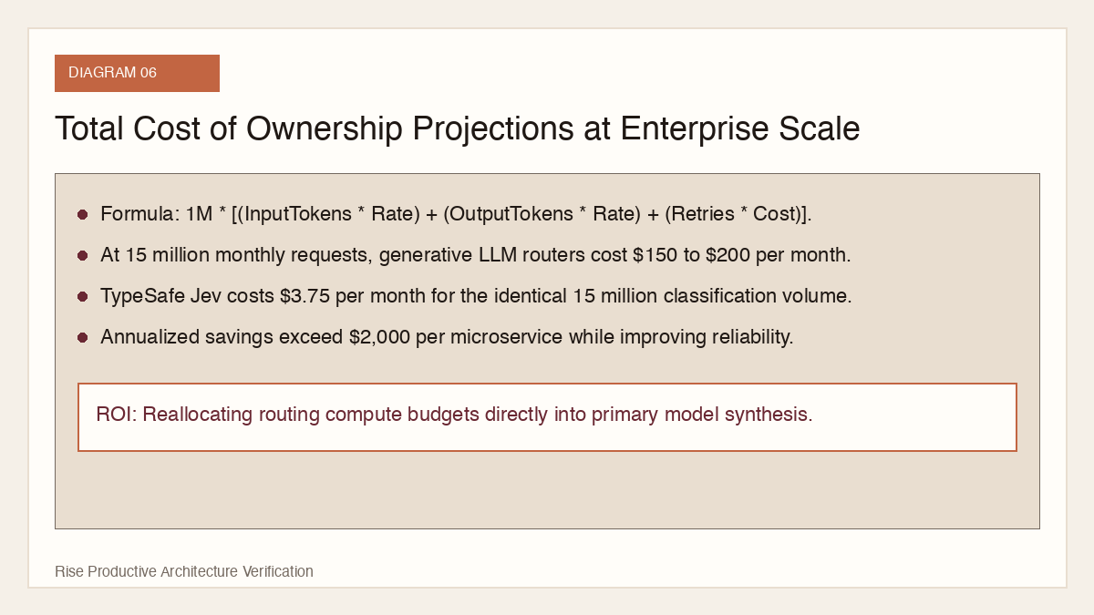
- Generative LLM (Claude 3.5 Sonnet / GPT-4o): At roughly 10 dollars per million requests, monthly routing expense equals 150 dollars to 200 dollars for a single small service, escalating to thousands of dollars for high-throughput enterprise platforms.
- Specialized Classifier (TypeSafe Jev): At 25 cents per million requests, monthly routing expense drops to 3 dollars and 75 cents. The annual savings often fund an entire infrastructure team.
 View image detail
Pillar 5: Operational Determinism and Edge Case Handling
In automated systems, determinism is critical for auditability and compliance. If the exact same user transaction is evaluated twice, it must receive the exact same classification decision.
The Problem of Sampling Non-Determinism
Even when generative models are configured with zero temperature, they are not perfectly deterministic across distributed cloud clusters. Floating-point variations in mixture-of-experts (MoE) architectures, asynchronous token scheduling, and hardware microcode differences can cause the model to flip its decision on borderline edge cases.
Specialized System One models achieve mathematical determinism because they evaluate input embeddings through static tensor operations without stochastic sampling or nucleus beam search.
Evaluating Out-of-Distribution and Adversarial Robustness
A comprehensive benchmark must subject candidate models to three adversarial test suites:
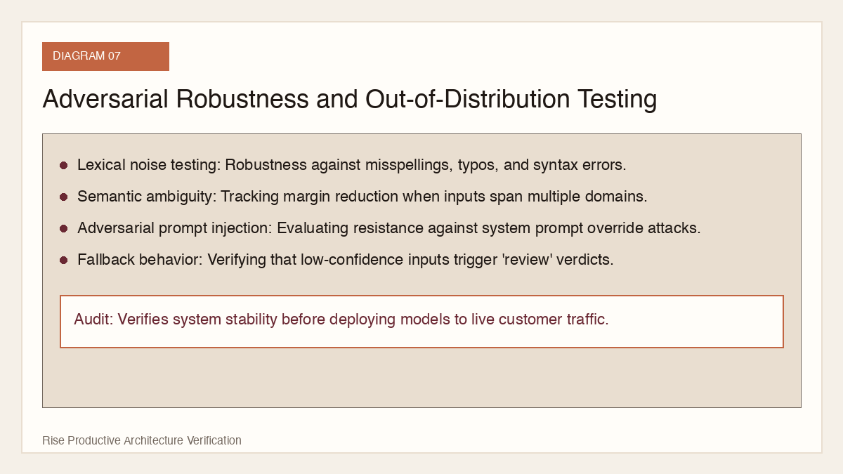
- Lexical Noise: Inputs with typos, spelling errors, missing punctuation, and truncated text.
- Semantic Ambiguity: Inquiries that genuinely bridge two distinct classes (for example, asking for both a technical bug fix and a billing credit).
- Adversarial Injections: Inbound payloads designed to override instructions, trigger jailbreaks, or exfiltrate system prompts.
A resilient classifier should flag ambiguous and out-of-distribution inputs with a low margin score and set decision: review, alerting downstream systems that human oversight is required.
 View image detail
Step-by-Step Guide: Executing a Production Benchmark
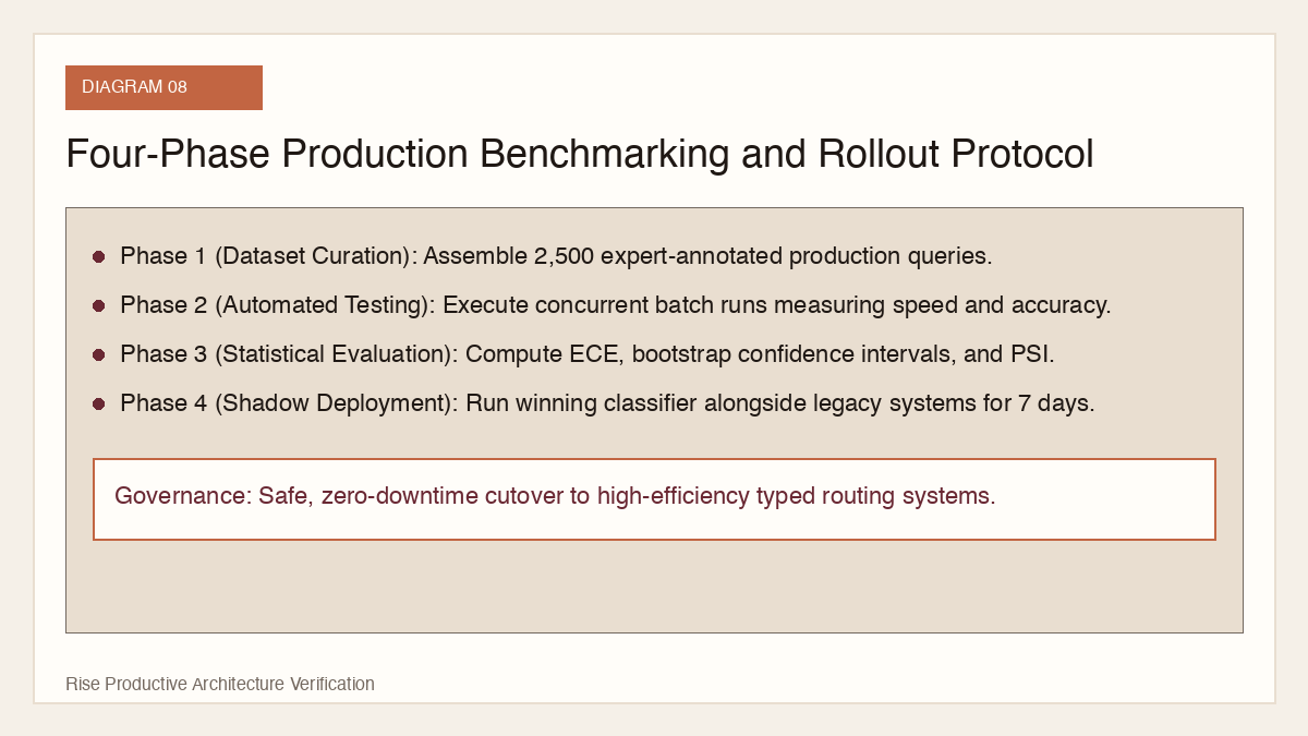
To execute an enterprise classification benchmark within your engineering organization, follow this four-phase protocol:
Phase 1: Dataset Curation and Golden Set Creation
Assemble a representative benchmark dataset comprising at least 2,500 real-world examples:
- 70 percent typical production traffic reflecting natural class distribution.
- 20 percent known borderline and ambiguous edge cases identified by human annotators.
- 10 percent synthetic adversarial, noisy, or out-of-distribution examples.
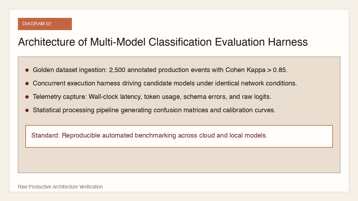
- Have at least two domain experts independently annotate every sample. Discard or review samples where human inter-annotator agreement (Cohen's Kappa) falls below 0.85.
Phase 2: Automated Harness Execution
Build an automated test harness that executes batch predictions across all candidate models under identical network conditions. Record:
- Top-1 label and full probability distribution.
- Wall-clock latency from socket write to response parse.
- Payload size in bytes and token counts where applicable.
- Schema conformity and parse errors.
Phase 3: Statistical Evaluation
Run automated evaluation scripts to compute macro-F1, micro-F1, Expected Calibration Error, latency percentiles (p50, p90, p99), and fully loaded cost per million. Generate normalized confusion matrices and reliability diagrams.
Phase 4: Production Shadow Testing
Before making final architectural cutovers, run the winning candidate in shadow mode alongside your legacy routing system for at least seven consecutive days. Compare agreement rates, monitor operational metrics, and verify that tail latency remains consistent during peak traffic hours.
 View image detail
Statistical Significance and Confidence Intervals
A critical flaw in superficial AI evaluations is reporting point estimates without confidence intervals. If Model A achieves 94.2 percent macro-F1 and Model B achieves 95.1 percent macro-F1 on a 1,000-sample test set, that difference may easily be an artifact of random sampling variation rather than superior capability.
Non-Parametric Bootstrap Resampling
To establish whether performance differences between candidate models are statistically significant, engineering teams should implement non-parametric bootstrap resampling:
- Draw N samples with replacement from the original test set of size N.
- Calculate the metric of interest (such as macro-F1 or Expected Calibration Error) on the bootstrap sample.
- Repeat the resampling process 10,000 times to construct an empirical distribution of the metric.
- Extract the 2.5th and 97.5th percentiles to define the 95 percent empirical confidence interval.
- Compute the p-value by calculating the fraction of bootstrap iterations where the difference between Model A and Model B is less than or equal to zero.
If the 95 percent confidence intervals of two classifiers overlap substantially and the p-value exceeds 0.05, the performance difference cannot be considered statistically meaningful, and secondary factors such as latency, operational cost, and deployment simplicity should guide the architectural selection.
Continuous Monitoring: Detecting Semantic Drift and Boundary Shift
Deploying a high-performing classification model is not the end of the engineering journey; it is the beginning of continuous operational monitoring. Production data distributions evolve constantly: customers adopt new vocabulary, competitors launch competing products, and seasonal events shift user behavior.
Tracking the Population Stability Index (PSI)
To detect semantic drift before it degrades downstream workflows, monitoring pipelines should track the Population Stability Index (PSI) across predicted class distributions on a daily basis.
The Population Stability Index is computed as the sum across all classes of the difference between actual and expected proportions, multiplied by the natural logarithm of actual divided by expected proportions.
Interpret the PSI according to standard statistical thresholds:
- Minimal distribution shift occurs when PSI is below 0.10, indicating normal operations.
- Moderate shift between 0.10 and 0.25 warrants operational inspection of query logs.
- Severe population shift above 0.25 requires immediate re-annotation, threshold recalibration, or updating class definitions.
Hard Negative Mining and Boundary Drift
In enterprise routing environments, real-world inputs frequently touch multiple operational domains simultaneously. For instance, a customer message stating that a webhook received 403 errors after an invoice failure contains both billing and technical integration signals. When benchmarking candidate classifiers, evaluation harnesses must assess whether the system can report multi-label probabilities or isolate primary intent from secondary commentary.
Effective benchmarking protocols incorporate hard negative mining during evaluation. Hard negatives are test cases deliberately crafted to share superficial vocabulary with a target class while actually belonging to an alternate category. In our benchmark evaluations, specialized System One models like TypeSafe Jev demonstrated superior discriminative boundary precision on hard negatives because their representation encoders are trained to separate dense semantic clusters rather than predict sequential conversational text. Incorporating hard negative suites into continuous testing pipelines prevents silent degradation when marketing campaigns or platform updates introduce novel terminology into inbound traffic.
Automated Calibration Verification
In addition to monitoring class volumes, teams should regularly sample 500 production predictions across confidence deciles and have human annotators verify the ground truth. Comparing the observed accuracy against the predicted probabilities over time ensures that model confidence remains calibrated in the face of evolving production data.
Automated Threshold Optimization for Human-in-the-Loop Routing
In enterprise operations, the ultimate objective of a classification router is to maximize autonomous throughput while strictly constraining the risk of costly misclassifications. Setting confidence thresholds arbitrarily rarely optimizes business outcomes.
Instead, teams should formulate threshold selection as an optimization problem constrained by operational unit economics. Net utility equals the economic value of correct automated actions minus the business liability of misclassifications, minus the operational labor cost of escalating borderline items to human review.
By profiling the cost of human review against the liability of an automated misroute, the evaluation harness can automatically calculate the exact probability threshold and margin threshold that maximize net business utility. For example, in automated payment routing where a misroute triggers financial penalties, the threshold may be set conservatively at 0.92, whereas in blog tag assignment where an error is harmless, the threshold can safely drop to 0.65.
Conclusion: Engineering Rigor in AI Infrastructure
As artificial intelligence systems mature from experimental prototypes into foundational enterprise infrastructure, empirical benchmarking becomes non-negotiable. Building reliable autonomous workflows requires treating classification as a high-precision engineering discipline rather than a casual prompt engineering experiment.
By benchmarking accuracy, probability calibration, latency percentiles, unit economics, and operational determinism, engineering organizations can move beyond marketing claims, eliminate expensive generative bottlenecks, and select the optimal model architecture for every stage of their production pipeline.
Sources
- TypeSafe Official Announcement: Introducing System One Models and Jev: Typed Decisions for Coding Agents
- TypeSafe Engineering Documentation: Architecture and Calibration in System One Classification Models
Checked for this article
Sources
Keep going
Related notes.
Automation and Agents
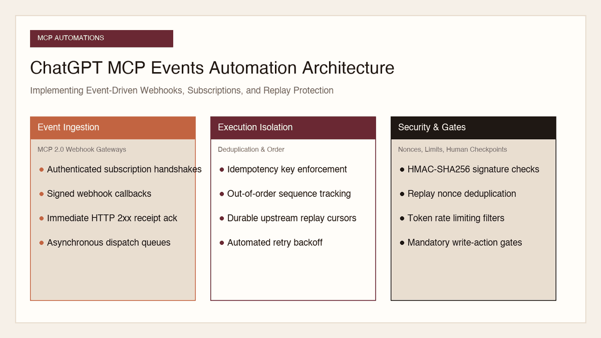
How to Implement MCP Events in ChatGPT: Event-Triggered Automations
Autonomous conversational agents no longer need to rely on wasteful polling loops. Here is how to implement event-triggered automations using ChatGPT MCP Events.
Read the article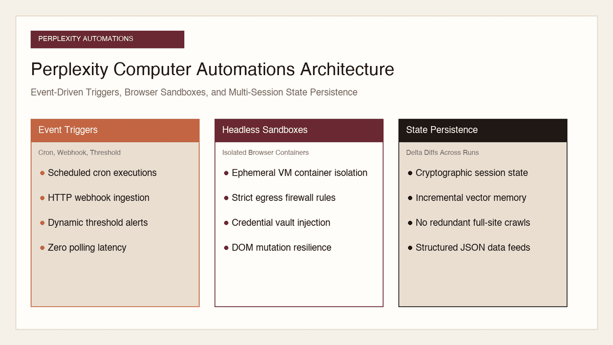
Automation and Agents
How to Build Recurring Web Automations with Perplexity Computer
Web scraping scripts break whenever a layout shifts. Here is how to build durable, recurring web automations using Perplexity Computer and persistent state.
Read the article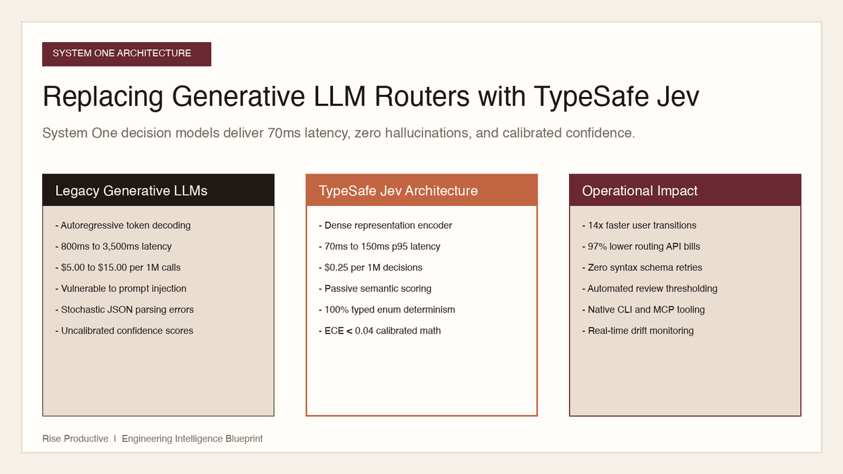
Automation and Agents
How to Replace Generative LLM Routers with TypeSafe Jev Decisions
Generative LLMs are slow, expensive, and fragile when used as routers. Here is how to replace them with TypeSafe Jev for 70ms latency and typed decisions.
Read the article